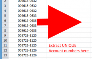
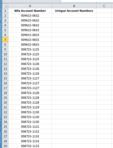
Suppose you have a spreadsheet at work and one of the columns contain a huge list of account numbers being exported from your company’s accounting system that contains a lot of duplicates. And you are tasked to extract the UNIQUE account numbers in this huge list.
If the list is just a short one, like 50 rows or 100, you can easily use the Conditional Formatting that highlights all duplicates, then you can manually delete the highlighted duplicates until no marked cells are left. This can be done easily with small list but if the list is as huge as 20,000 rows or 200,000 rows, the manual thing using Conditional Formatting will take forever to finish.

It is a good thing that Excel has a built-in way to extract unique data in a huge list of duplicates. The entire process is described below. I am using Excel 2010 so the screen shots provided are Excel 2010. If you are using Excel 2007 or 2013, I am sure it will also work.
How to Extract Unique Values in a Column
Open the Excel file to show the column that contains the data with duplicate.ô

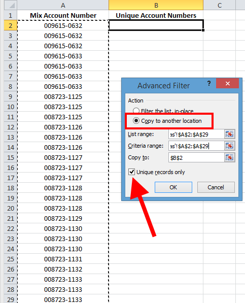
Click on theô Dataô tab, then click onô Advancedô under theô Sort & Filterô group.

In the Advanced Filter dialog box that opens, select “Copy to another location” under the Action group.
Under the List Range, click the mouse pointer there or click the button with the small arrow at the end of the box to minimize the dialog box and you can freely select the range with your mouse. Select the entire data range, the source of the duplicate data that you want to extract unique data from.
Do the same for Criteria Range.
For the Copy to box, click on the cell in another column where you want to start copying the unique account numbers to. In my case, I used B2.
IMPORTANT: Make sure to select the option that saysô “Unique records only”.

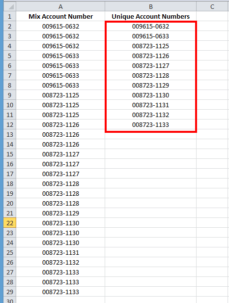
When you click OK, all unique data or records from the select list or range will be copied to B2 as shown below:

That is it! If you have questions, post them in the comment section.
